Cuda Programming

Introduction

This article presents an overview of the key learnings from an elective course titled "Programming on Massively Parallel Systems" offered at my university. The course is designed to impart comprehensive knowledge and practical skills in parallel programming, specifically utilizing Nvidia's CUDA (Compute Unified Device Architecture) framework.

The curriculum is structured around the paradigm of transforming sequential algorithms into parallel counterparts to enhance performance and efficiency. Central to this transformation is the CUDA API, which provides the necessary tools and architectural understanding to leverage Nvidia GPUs for computational tasks.

In this course, we delved into the intricate architecture of Nvidia GPUs, comprising streaming multiprocessors (SM), grids, blocks, warps, and threads. Understanding this architecture is crucial as it forms the backbone of effective parallel programming strategies.

One of the pivotal learning outcomes was developing a mindset for parallel thinking. This shift from traditional sequential processing to parallelism is not trivial; it involves a strategic approach to problem-solving. We explored the concept of parallelizability of problems, examining the dependencies within data and strategizing on optimal execution paths. This also included handling complexities and potential pitfalls associated with parallel execution.

The course's relevance extends beyond academic curiosity, particularly in the current technological landscape where AI and machine learning are at the forefront. Parallel programming, as taught in this course, is a critical skill in addressing the computational demands in these fields. It enables the handling of extensive data sets and complex algorithms that would otherwise be constrained by the limitations of standard CPUs.

While the course included three projects, I will focus only on the second project as it captures the skills learned as well as the power of writing effective CUDA code.

Project 2 Report

In this report, I detail the optimizations implemented in the spatial distance histogram (SDH) calculations. Our enhanced methodology involves two distinct kernels. The PDH Kernel manages the computation of distances, formulates, and creates private histograms in shared memory, and subsequently transfers these histograms to global memory. Following this, a secondary reduction kernel retrieves a private histogram from global into shared memory, applies a reduction algorithm on the buckets, and consolidates the data into a final histogram in global memory, which is then compared with the CPU results. This refined approach augments the efficiency of our SDH computations.

PDH Kernel

The PDH kernel is responsible for the large majority of the work in project 2.

Each thread in every block will contain an atoms data.

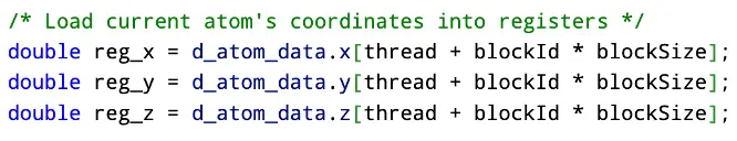
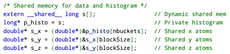
Due to the value being stored in registers, the access time for this data is roughly one clock cycle. Next is the process of setting up shared memory for every block to utilize quick access times to data. Since the size of shared memory would not be determined until run time, shared memory was allocated for each block in an external way. Here each block will have a private histogram as well as three lists that correspond to the x, y, and z atom coordinates. Shared memory typically has a size of 48KB on modern GPUs. Every block in the first kernel has

Assuming that in the worst case, nThreads is 1024, and we have 500 buckets,

This number is well under the 48KB size of shared memory.

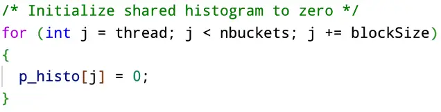
We set every value in the private histogram to be zero.

In the following section, each block, starting with itself, will load the next block into shared memory. This will allow for very quick access times when it comes to calculating distances. After the R’th block is loaded, the distances from all the points within L are calculated and added to the private histogram.

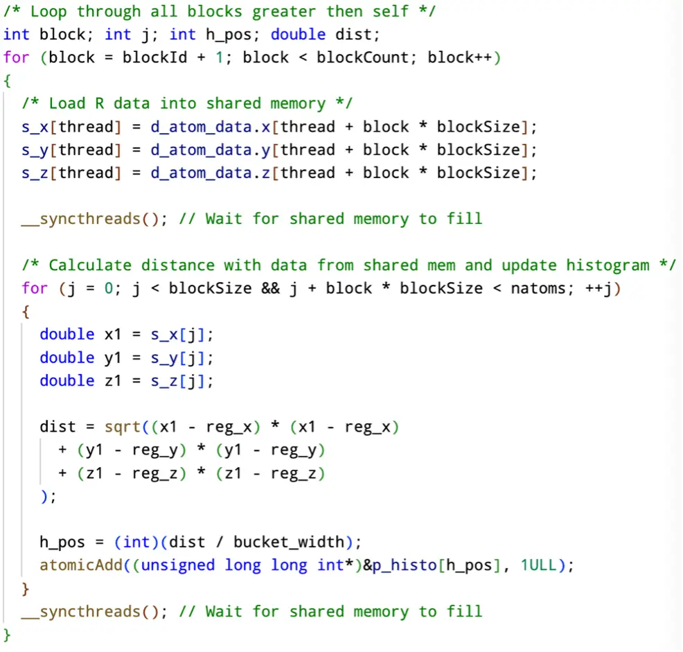
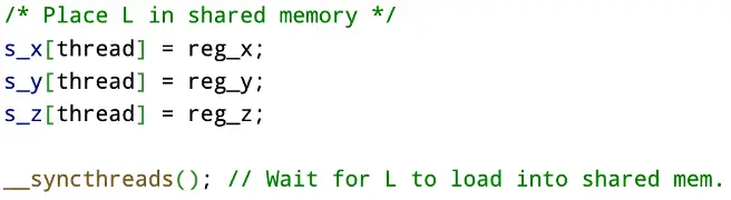
After every R’th block has been loaded and the distances have been calculated, the only distances left to calculate are those within itself. To do this, every block places it’s associated value from L into shared memory for all other threads of the same block to access.

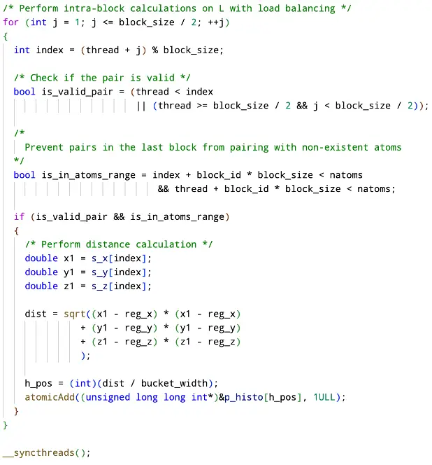
We perform the intra-block calculations with the help of load balancing to prevent thread divergence. Something important that we have to check is that a pair of atoms make a valid pair. A valid pair of atoms is when the two atoms are not the same and atoms are only computing distances that have not already been calculated. Additionally, we only want to count atoms that are in our range of atoms. This is more so important for the last block as the number of atoms may have not completely filled shared memory for that block.

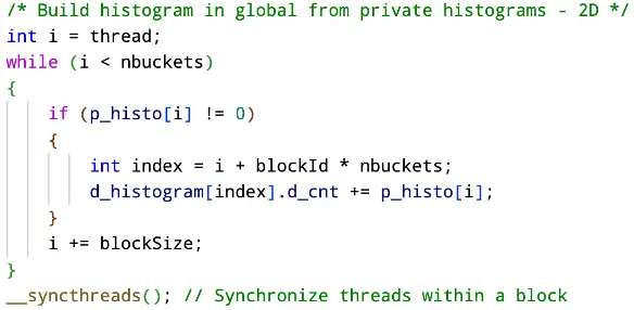
Finally, every block will take the data it has collected over the course of the previous steps and update global memory with the private value. This can be done without atomic instructions because instead of having every block competing to fill in the same buckets for a single histogram in global memory, we have the blocks update private copies in global memory. This will allow us to write a reduction kernel that can perform a sum reduction for every bucket in every block.

PDH Reduction Kernel

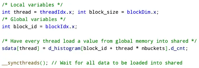
With every block having a private histogram in shared memory we can perform a parallel reduction algorithm on all the columns. We choose the columns because every column represents the same bucket number from all the blocks. This also means that we will have a total of bucket-count blocks. Also, there will be a bucket for every block we have, thus we have a total of block-count longs in shared memory for each block.

Again, since the size of the blocks are not known until runtime, we have to extern shared data.

The first step is to load every bucket from that column into shared memory for the block.

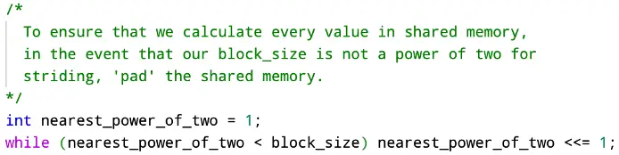
Since our thread count is designed to have one thread per row (block) of the column, we have to in a way pad our shared memory so that every value is counted in the striding. We get the closest power of 2 for each block that will determine our stride.

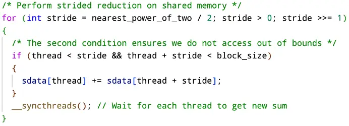
Then we actually perform the stride on shared memory.

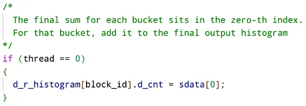
Finally, with the total count of n’th bucket siSng in the zeroth position of shared memory, we place that value into our result array for that block id. We can use the block id because for every bucket in our final histogram we have a block in the kernel.

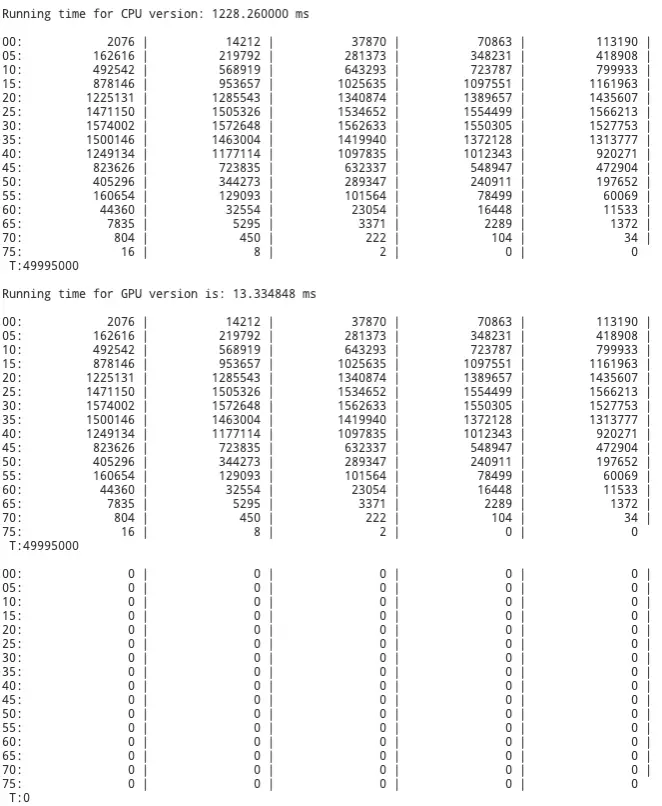
The resulting histogram is than compared with the final histogram.

Results

Looking at project 1 scores we see that the previous GPU version had a total run time of 53.25085 milliseconds.

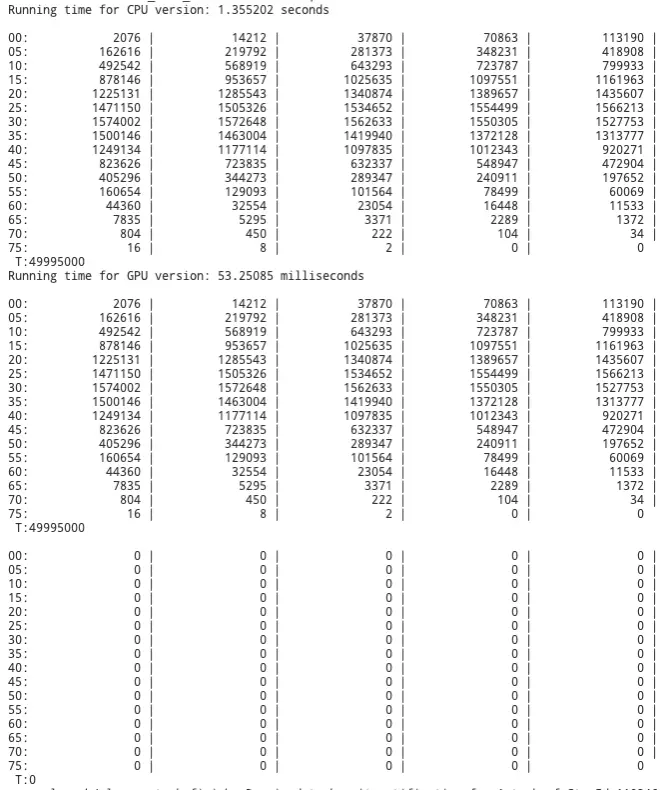
The new version of the GPU program shows to be 4x faster then the original program. Some tests even showed times of 10 milliseconds, which would be a 5x speedup from the first version of the GPU program. I say some tests because for some moments the program will run very fast 10-13 milliseconds. While other moments, when the system is most likely busy, the program can run as slow as 19 milliseconds.

Conclusion

The results of this experiment show dramatic improvement over the first version of the GPU program regardless; However, the exact improvement is hard to determine as the testing environment is bogged down by the number of users accessing it for GPU computation. The fastest reported time I received for the above algorithm was about 10 milliseconds. In comparison to the previous GPU program, the new version can push a speedup of 4-5x faster. But again, without an isolated testing environment it is difficult to determine the accuracy of these tests. Regardless, because of the utilization of shared memory, privatization, the stride reduction algorithm, and other CUDA techniques there is an obvious improvement from the first project.